2026-02-07

TL;DR: Noisy timing makes STDP thrash. In Part 1 we added uncertainty intervals. This post takes it to the next level and uses uncertainty as a signal to determine how much each neuron is willing to learn. When things are noisy, neurons freeze up. When the signal is good, they keep learning. No global tuning required.

The Barn Owl Problem

A barn owl hunts in darkness. It finds a mouse by comparing when a sound reaches its left ear versus its right ear (interaural time difference). The difference is on the order of microseconds. From that little difference, its brain computes a bearing and the owl dives.

On a quiet night, the signal is clean and the owl gets dinner. Bad night to be a mouse.

On a rainy night, every raindrop hitting the barn roof sounds like a mouse. Great night to be a mouse.

If the owl dove at every little ambiguous rustle, it would waste all its energy and catch nothing. So it doesn’t. When the signal is messy, the owl stays. The mice live.

In TrueTime meets STDP, we gave STDP the ability to know when spike timing is uncertain. With this post, we take it a step further:

Once you have uncertainty intervals, you don’t just get a better STDP update. You get a signal that tells you how plastic each neuron should be.

This takes us from “learning with uncertainty” to “staying stable under uncertainty.”

STDP in the Rain

With pair-based STDP, we’re trying to figure out if pre fired before post.

• \(\Delta t > 0\) means pre before post, so strengthen the synapse (LTP)
• \(\Delta t < 0\) means post before pre, so weaken it (LTD)

If timestamps are accurate, it works. If they’re not (say, because you’re crazy and built a system to spike neurons over a network) the synapse starts thrashing:

• sometimes your measurement says “pre before post”
• sometimes it says “post before pre”
• and the weight bounces back and forth

This is the owl diving at raindrops. Every rustle triggers a full send in one direction or the other. The synapse takes a random walk through weight space. The mice are safe, but only because the owl is spending all of its energy on nonsense.

In a small toy system this looks like “it won’t converge.” In a big system it looks like “everything gradually turns to soup.”

Nothing is Certain

With iuSTDP we stop pretending we know exact spike times. Each spike comes with bounds:

• pre spike: \([L_\text{pre}, U_\text{pre}]\)
• post spike: \([L_\text{post}, U_\text{post}]\)

Instead of “the mouse is at exactly 27 degrees”, the owl’s brain says “somewhere between 20 and 34 degrees” (he mouse would prefer a wider interval). That gives us three situations:

Certain order. If \(U_\text{pre} < L_\text{post}\), then pre definitely happened before post. Safe LTP. If \(U_\text{post} < L_\text{pre}\), post definitely happened before pre. Safe LTD.

Overlap. If the intervals overlap, you can’t really say who fired first. That overlap case is exactly where vanilla STDP amplifies noise.

Two Hunting Strategies

The first post has two ways to handle overlap:

Conservative mode. Only learn when order is certain. This is the “I refuse to learn from rumors” approach. It’s very stable (too stable). It usually means it doesn’t learn when things are slightly noisy.

Probabilistic mode. Always learn, but scale updates by confidence. This is the “I’ll adjust what I think, but proportional to how sure I am” approach. It avoids the brittle threshold of conservative mode.

Probabilistic mode seems to work better, but it’s still pretty bad.

The Drift Trap

Probabilistic learning drifts under ambiguity. Lets say we have a probability \(P\) that pre happened before post:

• \(P \approx 1\): pre-before-post is almost certain (LTP)
• \(P \approx 0\): post-before-pre is almost certain (LTD)
• \(P \approx 0.5\): you really can’t tell (shrug)

When \(P \approx 0.5\), the right thing to do is nothing. So we want ambiguous timing to produce minimal updates. But, that property isn’t automatic.

A simple way to get it done is to convert probability into signed evidence:

• \(s = +1\): definitely LTP
• \(s = -1\): definitely LTD
• \(s = 0\): no clue

Drive updates with \(s\) and the zero-evidence case produces no change. Problem solved.

Confidence as a Control Signal

But, we can still take it further. Once you have \(P\), you can define a confidence:

• \(c = 1\): very sure about the ordering (either direction)
• \(c = 0\): totally ambiguous

This is a measurement of how informative the timing evidence is in that region of the network.

And that means neurons can self-regulate:

• “I’m seeing clean causal evidence. I can learn quickly.”
• “I’m seeing ambiguous timing. I should slow down or freeze.”

Use confidence to decide how plastic a neuron should be.

This is the owl on the rafter. It doesn’t consciously decide “it’s raining, I should stop hunting.” Its auditory circuits just stiffen when recent signals have been ambiguous. Plasticity becomes local and self-tuning. No global learning rate schedule required.

Deterministic Islands

If you’ve been following the timing-as-data story, you know the tension.

Timing-coded circuits and the half-adder need stable timing. The whole point of those circuits is that information lives in when a spike arrives, not whether it arrives. If STDP rewrites the weights that control carry propagation timing, the adder breaks.

But on the other hand, recognition systems (e.g. the classic intro to neural networks handwriting tutorial) need a lot of plasticity.

If you train everything with STDP everywhere, the stable parts eventually get dragged around by the plastic parts. A confidence-based plasticity governor gives you a way to get both:

• where timing is clean and repeatable, learning can be strong
• where timing is messy, learning backs off automatically
• when the system becomes uncertain, plasticity drops so the network doesn’t rewrite itself

It’s the same philosophy as external-consistency in distributed systems: don’t commit changes when you don’t know what’s true. Here “commit” means “change weights.” If you’ve read the world brain post, this is one concrete piece of how a planetary immune system could protect itself.

How the Governor Works

Think of each neuron as having a plasticity knob, \(g\), between 0 and 1.

• \(g = 1\): fully plastic
• \(g \approx 0\): mostly frozen

On each spike pairing, the neuron measures confidence \(c\). It keeps a slow moving average: “have my recent pairings been trustworthy or ambiguous?”

When recent confidence is low, \(g\) drops. When recent confidence is high, \(g\) rises.

Instead of picking learning rates by hand, you let timing reliability tune it. This is the stabilizer layer that sits on top of iuSTDP. It’s the owl’s rafter patience.

Simulation

Here’s a toy simulation of what happens as timing jitter increases. Moving right on the x-axis, the question “did pre really fire before post?” gets harder to answer.

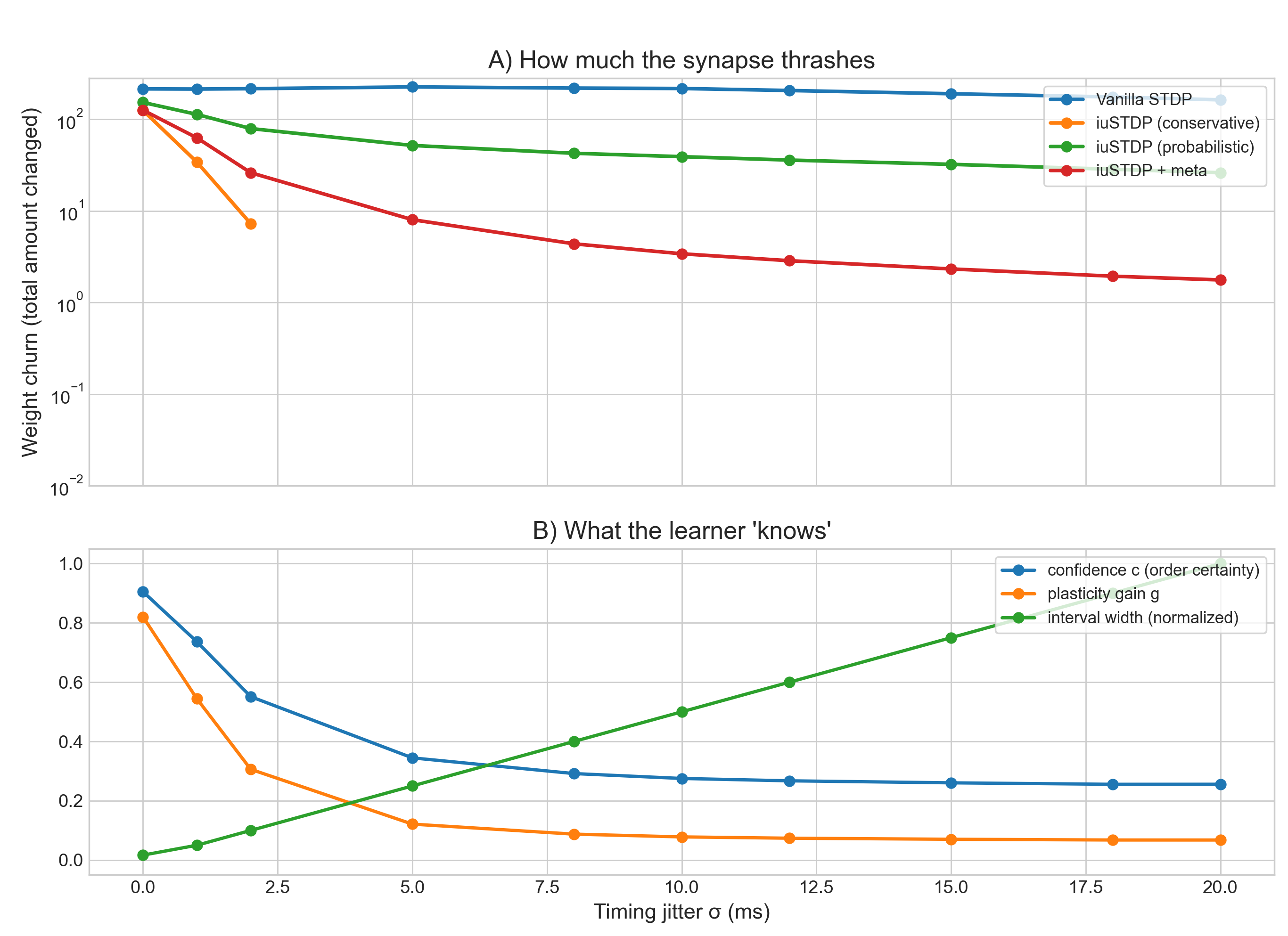
Panel A plots weight churn – the total amount the synapse weight changes over the run (log scale). Lower is better. It means the synapse is stable instead of being rewritten by noise.

Vanilla STDP (blue) stays high across all jitter levels. It uses point timestamps and commits to LTP or LTD based on a noisy coin flip, so it keeps making big updates even when the timing signal is garbage. It learns the noise and churns.

Conservative iuSTDP (orange) drops fastest. It only updates when the intervals don’t overlap, so the ordering is provably certain. When jitter is large, those certain cases become rare and churn collapses.

Probabilistic iuSTDP (green) sits in between. It still updates continuously, but scales updates by how likely the ordering is. Ambiguity produces smaller changes than vanilla.

iuSTDP + governor (red) is the practical compromise. It keeps churn far below vanilla across high jitter without requiring a hard “only learn when perfectly sure” rule.

Panel B explains why the curves separate. It shows what the learner “knows” about its own uncertainty.

Interval width (green) increases with jitter. Spikes are represented as time ranges, and bigger ranges mean less precise timing information.

Confidence (blue) decreases with jitter. Recall \(c = |2P - 1|\). When timing is ambiguous, \(P \approx 0.5\) and \(c \approx 0\): “I don’t know the order”.

Plasticity gain (orange) decreases even more sharply. It’s the slow, self-tuning knob derived from recent confidence. When jitter is high, \(g\) collapses and prevents the network from making large weight updates.

As timing becomes unreliable, the learner automatically shifts from “always update” (thrashing) to “update cautiously or not at all”. Stability is preserved.

What the Owl Can’t Do (Yet)

The governor tells the owl when to learn. If it’s a quiet night with clean signal, let’s dive and refine the hunting map. Loud night, ambiguous signal? The tree is a comfy place to hang out. The mice like the rain.

But the governor doesn’t tell the owl what to learn.

Right now, every clean pre-before-post pairing gets reinforced equally. The owl refines its internal map on every dive, including the ones that miss. It doesn’t distinguish “I dove and caught a mouse” from “I dove and smashed my face into the dirt”.

In biology, there’s a third signal. When the owl catches prey, a burst of dopamine washes through its auditory circuit and consolidates the recent synaptic changes. When the owl misses, those changes fade. Reward-modulated STDP is a three-factor learning rule where the third factor is a “yes, that worked” signal.

This works using eligibility traces. A spike pairing creates a temporary little bookmark at the synapse that says “this connection could change”. The bookmark decays over a few hundred milliseconds. If a reward signal arrives while the bookmark is active, the change is consolidated into a weight update. If no reward comes, the bookmark fades and nothing is updated.

Combine that with iuSTDP and you get a four-factor rule:

1. Timing evidence – did pre fire before post? (the STDP term)
2. Timing confidence – how sure are we? (the iuSTDP governor)
3. Eligibility – is the synapse still bookmarked? (the trace)
4. Reward – did the outcome matter? (the modulatory signal)

The governor filters out unreliable pairings. The reward signal filters out irrelevant ones. Together they answer both “should I learn right now?” and “is this worth learning at all?”

That’s the next post. The mice should be worried.

Napkin Math

I’m sure I made a billion mistakes here, but the overall concept seems sound.

From Intervals to Mean and Uncertainty

Spikes:

• \(t_\text{pre} \in [L_\text{pre}, U_\text{pre}]\)
• \(t_\text{post} \in [L_\text{post}, U_\text{post}]\)

Midpoint estimate:

where:

Approx. uncertainty assuming each interval is uniform:

Let \(w_\text{pre} = U_\text{pre}-L_\text{pre}\), \(w_\text{post} = U_\text{post}-L_\text{post}\).

(You can add extra terms for jitter or clock uncertainty if you feel like it)

Now model:

Causal Order

where \(\Phi\) is the normal CDF.

Signed Evidence and Confidence

Signed evidence:

Confidence:

So:

• \(P=0.5 \Rightarrow s=0 \Rightarrow c=0\) (ambiguous)
• \(P \to 1 \Rightarrow s \to 1 \Rightarrow c \to 1\) (certain LTP)
• \(P \to 0 \Rightarrow s \to -1 \Rightarrow c \to 1\) (certain LTD)

Probabilistic Update

To ensure ambiguous evidence doesn’t drift, use a symmetric timing kernel:

Properties:

• If \(P=0.5\), then \(s=0\) so \(\Delta w=0\).
• If evidence is confident, \(|s|\) is large and the update grows.
• Timing farther apart (large \(|\mu|\)) produces smaller updates.

Plasticity Governor (e.g. metaplasticity Gain)

Maintain a slow confidence average per postsynaptic neuron \(i\):

Convert this into plasticity gain:

Finally gate learning:

• \(\gamma > 1\) makes the neuron “freeze unless confident”.
• \(\alpha\) controls how quickly the neuron reacts to changing uncertainty.

Related

Three-factor learning rules. Izhikevich (2007) and Fremaux & Gerstner (2016) established that STDP + eligibility traces + dopamine solves the distal reward problem. The four-factor rule sketched above adds a confidence gate on top of their three factors.

Berthet et al. (2016). The term “four-factor learning rule” exists, but their fourth factor is dopamine receptor type (D1 vs D2), not a confidence signal.

The Synaptic Filter. Jegminat & Pfister (2020) track uncertainty about the weight itself and use that to modulate learning rate. Kinda close to the confidence governor. They ask “how sure am I about this weight?” while iuSTDP asks “how sure am I about the evidence?”. Maybe they can be merged.

BCM theory and metaplasticity. The governor resembles the sliding threshold in BCM theory (Bienenstock, Cooper & Munro 1982) and the general concepts in metaplasticity (Abraham & Bear 1996). But, BCM tracks firing rate and shifts the direction of plasticity. The governor tracks timing quality and scales the magnitude.

Google TrueTime and Spanner. The interval idea comes from distributed systems. TrueTime (Corbett et al. 2012) gives you a time interval instead of a timestamp. Spanner won’t commit a transaction unless it can prove the ordering. iuSTDP applies the same logic to spike timing.